Human-In-the-Loop Data Collection
Testing human-in-the-loop data collection on a real robot: when to step in, how to intervene, and whether it beats just collecting more demonstrations.
Human-In-the-Loop (HIL) data collection promises to improve a policy by demonstrating how to act in the situations where it struggles. Instead of collecting more data everywhere, you spend your effort exactly where the policy is weak, which should be a time-efficient way to reach a high success rate. I wanted to test this out for myself during my time at Dream Machines, and work out how to get the best results out of it.
Questions
When I first read about HIL data collection in the π*0.6 paper, the concept seemed simple and made a lot of sense: you improve a policy by collecting more data in the situations where it struggles. Easy! But once I wanted to do it myself, I realised it needed a bit more thought. It wasn’t quite that simple.
The data is usually collected by rolling out a policy while a human watches, stepping in whenever it struggles to demonstrate how to act in that situation. This data then trains the next iteration of the policy, which ideally performs better than the last. A prerequisite is a setup that lets you smoothly take over control from a running policy, so I implemented VR teleoperation for our setup at Dream Machines (more on that in my previous blog post: VR teleoperation stack). Even with that in place, I had several open questions about how to get the best results:
- When exactly should I stop the policy?
- How should I do the interventions?
- How many interventions should I do before training a new policy iteration?
- Do I fine-tune the previous policy with the new data, or train a new policy from scratch on the aggregated dataset?
To find answers, I started by reading about the topic.
Background
The idea of iteratively aggregating data and improving policies goes back to 2010, when Ross et al. introduced DAgger (Dataset Aggregation). Their goal is to imitate the behaviour of an expert, which is simply whatever provides the correct action, be it a policy, an algorithm, or a human. Instead of training the policy only on the states the expert visits during demonstrations, DAgger also trains it on the states the still-imperfect policy visits itself. The policy is rolled out to decide where to go and the expert is queried for the correct action at each visited state. The experts actions in the states explored by the policy is aggregated with the original dataset to train the next iteration. The policy’s own actions are only ever used to act and explore the state space, never as training labels.
HG-DAgger (Human-Gated DAgger) uses a human as the expert, which decides when to intervene. Instead of querying the exper at every state, a person watches the rollout and decides when to take over to demonstrate the right behaviour. Only the interventions are then aggregated with the initial demonstrations, and each new policy is retrained from scratch on this data (no fine-tuning).
HIL-SERL collects data the same way as HG-DAgger but uses it differently: instead of plain behaviour cloning, it optimises the policy with off-policy reinforcement learning, splitting the intervention data between a demonstration buffer and an RL buffer that are weighted differently during training. As the policy reaches higher success rates and faster cycle times, the human gradually intervenes less.
While the previous paper don’t specify how the interventions are done exactly, RaC (Recovery and Correction) introduces two rules about that:
- When the policy makes a mistake, first recover into in-distribution states, then correct and finish the subtask.
- End the rollout right after the intervention, so the data never contains states produced by a mix of policy and human control.
They show this is more data-efficient than HG-DAgger: the policy learns to recover and try again, which raises the success rate (at the cost of a longer average time on the successful episodes).
π*0.6 aggregates its data in an improvement loop of autonomous rollouts where expert operators step in to correct catastrophic failures and recover from mistakes. They don’t spell out the details (no explicit recover-then-correct rule, and no mention of when an episode ends), and they fine-tune each iteration from the pre-trained checkpoint rather than from the previous one.
Finally, the LeRobot docs have a practical section on HIL data collection. They advise intervening when the robot is about to make an irreversible mistake, hesitates, or deviates from the expected trajectory. They recommend RaC’s first rule (recover, then correct) but not the second (they don’t terminate after an intervention but rather give control back to the policy and continue). They also fine-tune the policies iteratively rather than retraining from scratch. But their code examples are only for , a much bigger policy for which retraining from scratch every iteration wouldn’t make sense anyway.
After reading all this, I settled on the following for my own experiments:
- Use LeRobot’s guidance on when to intervene.
- Recover into in-distribution states before correcting (RaC’s first rule).
- For small policies like mine, retrain from scratch on the aggregated dataset.
- Continue the episode after an intervention rather than terminating after the first one (so, not RaC’s second rule).
Experiment
With these decisions made, I planned a set of experiments to see whether I could actually get useful results out of HIL data collection. I chose to train ACT policies, since they are small enough to train locally and I already had a working configuration and some experience with them (more on that in my previous blog post: First Week of Imitation Learning). I started by finding a good training configuration for the task, which I would then reuse throughout. The main question was whether collecting intervention data beats simply collecting more demonstrations of the full task. While running that comparison, though, I realised I still wasn’t sure how exactly the interventions should be done, so I added a third experiment comparing different intervention styles. The three experiments ended up being:
- Experiment 1: find a good ACT training configuration for the task.
- Experiment 2: compare collecting intervention data against collecting more demonstrations.
- Experiment 3: compare different intervention styles.
I used a small cube pick-and-place task with three increasingly difficult subtasks (figure 1). I kept the task rather simple and short, such that I can iterate more quickly. For evaluation I scored each episode by its task progress, recording the last subtask it finished successfully. This also lets me recover the overall success rate.
Progress score:
- 0.3: Pick up a cube on the left half of the table.
- 0.6: Hand the cube over to the right hand.
- 1.0: Place the cube into the square slot.
Every policy evaluation in the three experiments are done with 32 episodes. More details about the task and the evaluation are in the Appendix.
Experiment 1: ACT Configuration
Goal: Find a good ACT training configuration for the task.
I took most of the parameters from my earlier ACT experiments (First Week of Imitation Learning), and for the batch size I used the largest that fit on our workstation. The one parameter really worth tuning for this task was the number of training steps, so I trained a single policy out to 320k steps and evaluated its checkpoints along the way.
Procedure
- Collect 100 demonstrations, creating the dataset .
- Train an ACT policy on up to 320k steps, storing intermediate checkpoints.
- Evaluate the checkpoints [6k, 10k, 20k, 40k, 60k, 80k, 120k, 160k, 320k].
Result
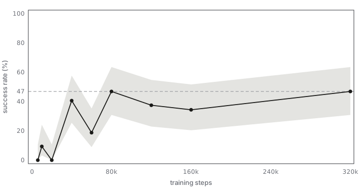
The success rate jumps sharply between 20k and 40k steps (0% → 41%) and then plateaus, peaking at 47% at both 80k and 320k steps (figure 2).
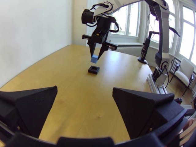
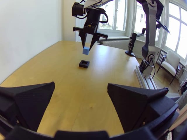
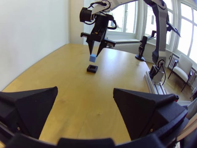
The policy also gets qualitatively smoother with more training, with cleaner transitions between action chunks. This is easiest to see at the early checkpoints (figure 3).
Take-Away
Even at 320k steps, which is more than 120 epochs over the dataset, the performance doesn’t degrade. I suspect the task is simple enough that the policy just doesn’t overfit. Since the 80k and 320k checkpoints are almost indistinguishable (if anything, 320k is a touch smoother), I went with 80k steps for all the following experiments. That takes about 6 hours to train on our local GeForce RTX 5090. The full training configuration is in the Appendix.
Experiment 2: Intervention vs Demonstration
Goal: Compare a policy trained on HIL intervention data against one trained on more demonstrations.
To make this comparison, I ran three rounds of data collection on top of the initial 100-episode dataset from Experiment 1. In each round I either collected 50 more full demonstrations, or rolled out the current policy for 50 episodes and intervened where needed, giving me two parallel branches of policies to compare.
For this experiment I corrected the policy after it made an error, that is, after it failed to place the cube into the slot. I recovered from the failure state (picked the cube back up), returned to an in-distribution state (holding the cube above the slot), and finished the subtask it had failed (inserted the cube). Figure 4 shows one such intervention.
Procedure
The steps in parentheses were already done in Experiment 1, so I carried their results over instead of redoing them. A superscript marks which branch a dataset or policy belongs to: I for the intervention branch and M for the branch that keeps adding more demonstrations.
- (Collect 100 demonstrations, creating the dataset .)
- (Train the base policy on for 80k steps.)
- For in [1, 2, 3], starting from and :
- More demonstrations: collect 50 new demonstrations and add them to , giving .
- Interventions: record 50 rollouts of with interventions and add the intervention segments to , giving .
- Train policy on and on , each for 80k steps.
- Evaluate all trained policies.
Result
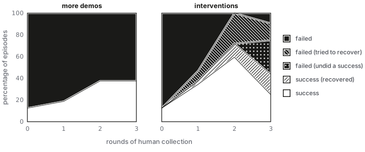
The policies trained on intervention data improve faster and reach higher success rates than those trained on more demonstrations alone (figure 5). The best success rate, 72%, comes after two rounds of intervention data. After a third round the policy starts to revert its own successful insertions, grabbing the cube again and then failing to re-insert it. These correction attempts mostly time out, running past the 60-second cap. The demonstration-only branch tops out at 38% after 200 episodes, and adding another 50 demonstrations doesn’t change that.
The interventions also got rarer as the policy improved. The share of rollouts that needed me to step in fell from 78% to 38% over the three rounds.
| round | rollouts | episodes w/ intervention |
|---|---|---|
| 1 | 50 | 39 |
| 2 | 50 | 29 |
| 3 | 50 | 19 |
Because only the segments where I was in control are added, the intervention dataset grows slowly. After three rounds it holds 187 episodes and 123,930 frames, against 250 episodes and 203,834 frames for the demonstration dataset, even though it produced the better policy.
| round | demo episodes | demo frames | intervention episodes | intervention frames |
|---|---|---|---|---|
| 0 | 100 | 80,831 | 100 | 80,831 |
| 1 | 150 | 119,285 | 139 | 100,151 |
| 2 | 200 | 162,498 | 168 | 113,930 |
| 3 | 250 | 203,834 | 187 | 123,930 |
Figure 6 shows four behaviours I saw at the third round: a clean first-try success, a successful recovery and correction, a reverted success, and a timeout.
Take-Away
Two things stand out. First, the comparison is clear: the intervention data used less actual data than the extra demonstrations, yet it raised the success rate more. Second, the interventions changed the policy’s behaviour, not just its score. After one round it barely attempted any corrections. After two rounds it tried to correct essentially every failure, though it didn’t always succeed.
The way I ran the interventions also produced the odd round-three result where the policy reverts its own successes. It never learned to reliably tell whether the cube was already seated, so it would re-grab a correctly placed cube and then fail the re-insertion. Had I stopped each episode the moment the cube was correctly inserted, the success rate after three rounds would even have been 75%.
It is also worth noting that the gains didn’t come only from corrections. First-try successes went up as well, from 13% for the base policy to 59% after two rounds of interventions. That is probably down to how I did the interventions: after recovering the cube I always moved back above the slot and demonstrated the insertion from there, which adds more data for the very first insertion attempt too.
One process note. At first I evaluated each policy right after it finished training, which meant the evaluations happened on different days, at different times, under different lighting. It turned out those conditions can change a policy’s performance quite a lot, so I redid all the evaluations back-to-back on a single day. This is also why the number of interventions per round in the table above deviates from the results during the evaluation. The numbers above are from that second round, and the first-round results are in the Appendix (figure 13). In that first round I saw only a single correction attempt from , and the over-correction, where the policy reverts its own successes, already showed up with . Together these made me question whether I was intervening the right way, which is what motivated the third experiment.
Experiment 3: Intervention Styles
Goal: Compare different intervention styles.
I compared four intervention styles:
nudge: stop the policy just before it fails and correct with a small nudge.redo: stop the policy just before it fails, rewind, and redo the hard part.recovery: let the policy fail, then recover, return to an in-distribution state, and correct.recovery+: let the policy fail, rewind a little while recording, then take over to recover, return to an in-distribution state, and correct.
The motivation for recovery+ came from that single correction attempt I saw after one round of recovery-style data. I suspected the problem was that taking over right after a failure drops the policy straight into states it has never seen. So with recovery+ I first rewind the last few actions, walking the arm back through states it actually normally passed through, and only then take over. Crucially, the rewind is recorded too, so the dataset contains a path from the failure back through familiar states, when the cube isn’t placed correct.
nudge and redo come from the opposite worry. Once the policy started reverting its own successes, I wanted to see how far I could get with interventions that only improve the first-try success and never teach recovery at all.
For each style I collected a single round of intervention data over 50 episodes. Figure 7 shows an example of each.
Procedure
- (Collect 100 demonstrations, creating the dataset .)
- (Train the base policy on for 80k steps.)
- For each style in [nudge, redo, recovery, recovery+]:
- Record 50 rollouts of with -style interventions and add them to , giving .
- Train on for 80k steps.
- Evaluate all trained policies.
Result
How much I had to intervene during collection, and how much data that added, varied by style. The intervention depth is the median fraction of an episode I spent in control, so a shallow depth means short interventions:
| style | rollouts intervened | intervention depth (median %) | intervention frames |
|---|---|---|---|
| nudge | 31/50 (62%) | 8% | 2,100 |
| redo | 35/50 (70%) | 34% | 9,049 |
| recovery | 39/50 (78%) | 39% | 19,320 |
| recovery+ | 26/50 (52%) | 40% | 14,877 |
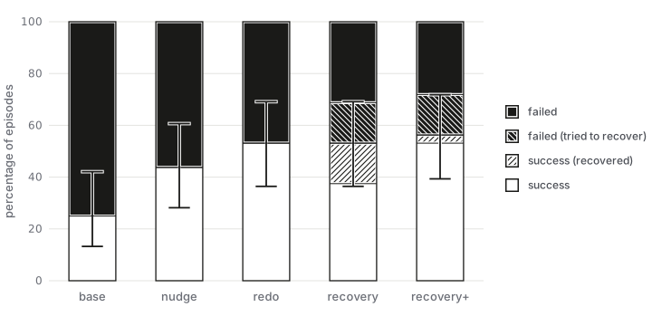
After a single round, recovery+ reaches the highest success rate (56%), with a lot of first-try successes (figure 8). recovery is close behind (53%) and makes many correction attempts, succeeding on roughly half of them. nudge and redo both improve on the base policy (25%), with redo (53%) ahead of nudge (44%).
Discussion
nudge beats the base policy but trails the other three styles. I think the reason is simply how little data a nudge adds: the corrections are so short that there isn’t much signal to learn a new skill, and it would probably need many more episodes. And since a fixed number of intervention episodes takes about the same time regardless of style, nudge also collects the least data per unit of time by a wide margin.
recovery+ gives the best results here, but it doesn’t really lend itself to more than one round. In the sections where I recorded the rewind to teach the correction, the resulting policy () sometimes hesitates, flickering between continuing and reversing (figure 9). Through the recorded rewinds, that hesitant behaviour would feed straight into the next round’s dataset, which isn’t what I want.
Comparing recovery and recovery+ on the episodes where the first insertion failed, recovery actually attempts a correction in more of them (in 31% of all evaluation episodes, versus 19% for recovery+). Since the two styles differ only in how the correction is started, this suggests the explicit rewinding isn’t necessary: simply letting the operator “rewind” by physically moving the arm back after a failure is already enough to elicit the correction attempts.
redo improves on the base purely by raising the first-try success rate, since it never teaches the policy to recover. Interestingly, recovery+ improved the first-try rate about as much as redo did. The same effect I described in Experiment 2, where always lifting the cube back above the slot before re-inserting adds data for the first approach too.
One thing I would change: I fixed the number of rollouts (50) per style rather than the number of interventions, so the styles don’t all rest on the same amount of intervention episodes (see the table above).
While watching and seeing how often it corrected, I went back to re-evaluate , which I had first evaluated a few days earlier (during Experiment 2’s first evaluation round) and where I had seen only a single correction. The re-evaluation looked completely different, with lots of corrections. The only visible difference between the two recordings is the light in the window. The first evaluation looks like it was recorded early in the morning, while the re-evaluation had bright sunlight coming through (figure 10).
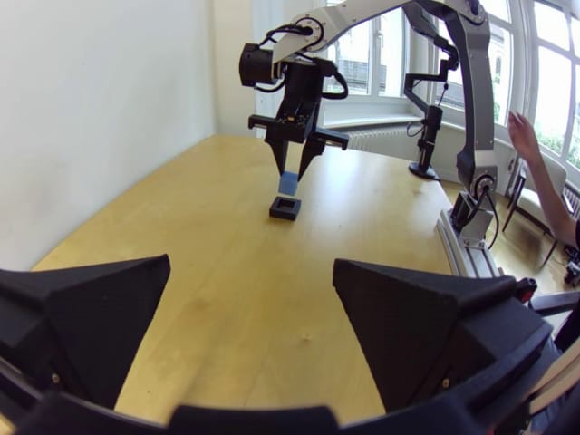
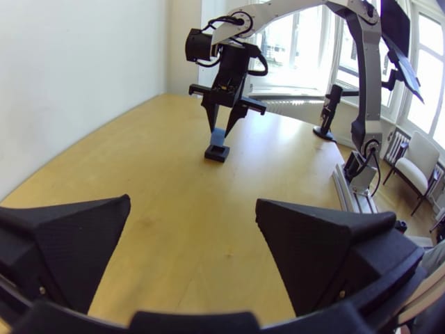
Because of that, I also re-evaluated the base policy to keep the comparison fair, and ran every evaluation for this third experiment back-to-back on the same morning under consistent light (figure 14 in the Appendix).
Conclusion
Across these experiments, HIL data collection did what it promised for the small ACT policy I trained. Spending the same time budget on interventions instead of extra demonstrations gave me a better performing policy, and it got there faster: the success rate climbed to 72% after two rounds of interventions, while collecting more full demonstrations plateaued around 38%.
But the experiments also showed that the details of the intervention matter as much as the decision to intervene at all. The same recover procedure that pushed the success rate up also taught the policy to second-guess itself: by the third round it would undo its own correct insertions. I think this comes from how I recorded the corrections. I stopped right after re-inserting the cube, so each correction ends on the insertion and never on leaving the placed cube alone and returning home. The original demonstrations do show that ending, but the corrections kept adding data for re-grabbing. Comparing intervention styles, the ones that demonstrate recovery (recovery, recovery+) gave the best results. recovery+ came out slightly ahead, but its recorded rewinds make it hard to iterate, and plain recovery got most of the way there.
So, to get the best results out of HIL data collection, here are my main take-aways:
- Recover into in-distribution states after a failure, then solve the failed part the same way as in the demonstrations. That teaches the policy to recover, and because the correction approaches the goal just like a demonstration does, it lifts the first-try success rate too.
- Additionally I would finish the whole subtask when doing a correction, instead of stopping the moment the cube is seated, so the policy does not overfit to correcting even when it has already succeeded.
About running the experiment itself, here is what I would do differently next time:
- Fix the number of interventions per round rather than the number of rollouts, so every round and style is compared on the same amount of intervention data (π*0.6 fixes the interventions this way too).
- Evaluate every policy back-to-back under the same conditions. This one wasn’t really about HIL at all, and it was the biggest surprise of the project: a change in daylight alone was enough to turn “one correction” into “lots of corrections” for the same policy.
- Choose a longer task with more subtasks. Even the base policy, trained on just the initial 100 demonstrations, cleared the first two subtasks every time, so the policies only ever differed on the final insertion. More steps that are not solved straight away would spread them across the progress score and make them easier to compare.
The questions I am most curious about now are about transfer. Would the same intervention recipe carry over to other tasks, and to other kinds of policies, especially the larger VLAs that are fine-tuned rather than retrained from scratch?.
Appendix
Task
The task used for the experiments is a small cube pick-and-place task with three increasingly difficult subtasks. The task is to:
- pick up a cube on the left half of the table,
- hand it over to the right hand,
- place it into a square slot.
Figure 1 shows a video of one demonstration of the task.
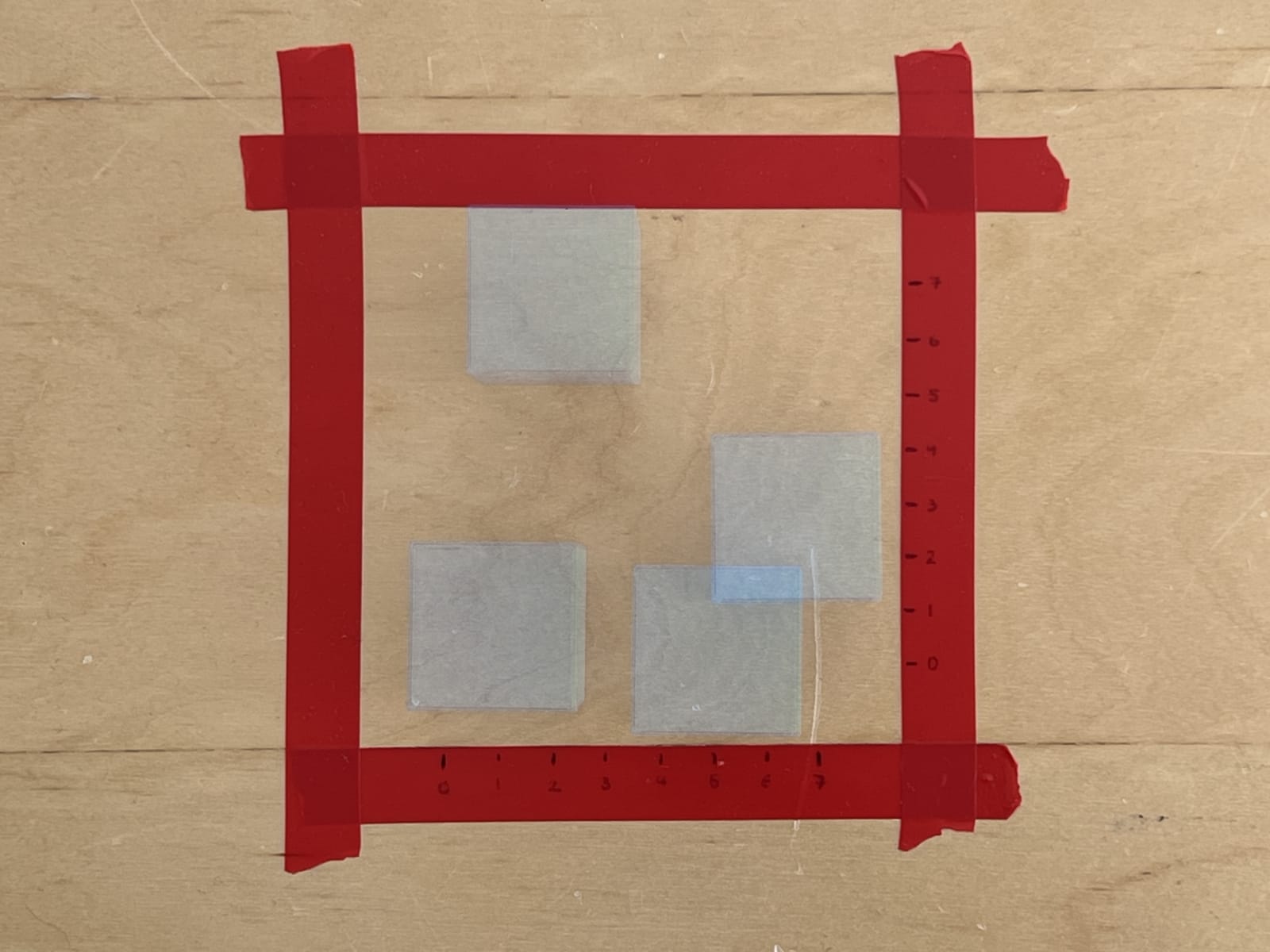
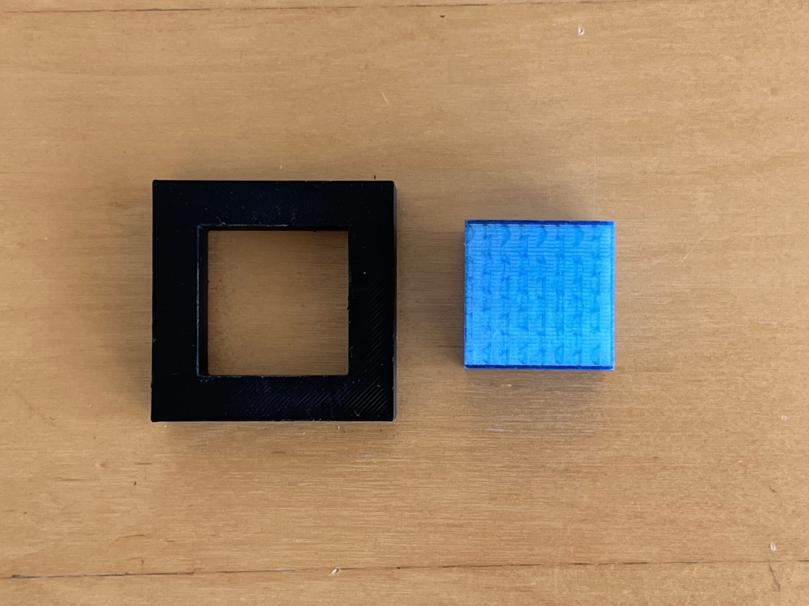
The cube is 30×30×30 mm. It is placed at a random position inside a marked 10×10 cm square, always in the same orientation (figure 11, left). The slot is 31×31 mm and always in the same location (figure 11, right).
Evaluation
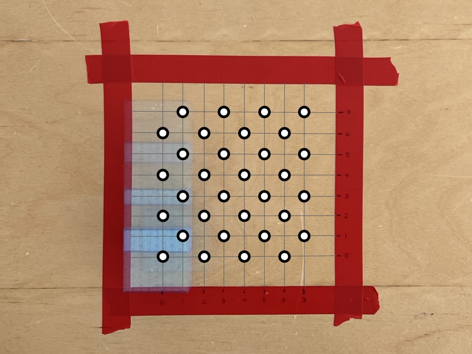
For evaluation I place the cube on an 8×8 grid of positions inside the 10×10 cm square, using every second grid cell, which gives 32 trials per policy (figure 12).
I rate each policy with the task-progress score: if it fails a subtask, it keeps the score of the last subtask it completed. The success rate then falls out of the scores, as the share of episodes that reach 1.0.
Progress score:
- failure: 0.0
- pick_up: 0.3 (the cube leaves the ground while in contact with both sides of the gripper).
- hand_over: 0.6 (the right gripper holds the cube by itself).
- place: 1.0 (the cube is fully inserted and correctly oriented in the slot, and the arms return to the rest pose).
On top of the score, the operator tags the failure mode during evaluation, which allows for a more fine-grained analysis afterwards.
I found it helpful to divide the task roughly into a small number of subtasks with a clear definition for each, so I don’t have to think about the score while evaluating. The failure-mode tags, on the other hand, are easiest to add live, since you only learn the exact failure mode by watching.
The operator stops the episode manually when the arms return to the rest pose, the policy gets stuck, or it makes an unrecoverable failure, and automatically after 60 seconds. A demonstration takes about 16 seconds on average, so the 60-second cap still leaves room for several recovery attempts.
ACT training configuration
chunk_size: 50n_action_steps: 50kl_weight: 10.0optimizer_lr: 3e-5optimizer_lr_backbone: 3e-5batch_size: 32steps: 80k
Experiment 2: Evaluation 1
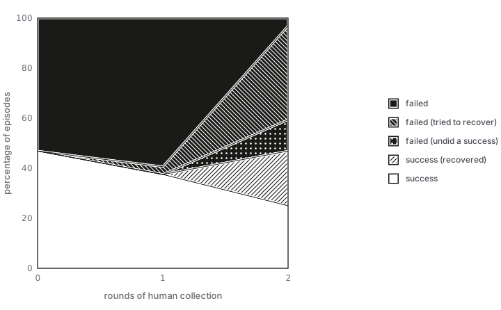
In Experiment 2’s first evaluation round, I evaluated each policy right after it trained, which meant different days and different lighting. The evaluation reuses the one from Experiment 1. Figure 13 shows the intervention branch across those rounds in the first evaluation: self-correction grows, but by the last round (round 2) a sizeable share of episodes time out or revert their own success.
Experiment 3 re-evaluation
After finding how much the lighting moved the results, I ran every evaluation for the third experiment back-to-back on the same morning, under the same light. Figure 14 shows the starting scene of episode 0 for each of the four style re-evaluations, which looks consistent across all of them.